Roger N. Shepard ,Toward a Universal Law of Generalization for Psychological Science.Science237,1317-1323(1987).DOI:10.1126/science.3629243

Starting from the seminal paper of Shepard (1987), I took a first glimpse of psychology as a quantitative science (like physics, which i love so much). The universality in the seemingly unpredictable, noisy behaviors is amazing.

Primacy of Generalization

Anything experienced by an individual is unlikely to recur in exactly the same form and context

• To make learning useful, one has to generalize.
• Each individual has an internal metric of similarity (exists at birth)

Generalization vs. failure of discrimination

Encountering an unfamiliar object requires the individual to infer the consequence

• Generalization is a cognitive act
• psychological vs. psychophysical

Early work

when Pavlov found that dogs would salivate not only at the sound of a bell or whistle that had preceded feeding but also at other sounds-and more so as they were chosen to be more similar to the original sound, for example, in pitch.

Empirical gradient of generalization: relate feature of response to some measure of difference

• strength, probability, speed etc.

Example. identification learning (Shepard, 1980)

• subjects learn a one-to-one association between $n$ stimuli and $n$ arbitrary verbal responses
• measure of generalization $g_{ij}$: the frequency with which any stimulus lead to response assigned to any other

Apparent noninvariance

To establish quantitative results, we have to choose a independent variable

• choosing physical measures of difference does not guarantee invariance
• the decrease in response has different patterns with various stimuli, sesory continuum, or species
• even exhibit nonmonotone increase: tones separated by an octave, hues at the opposite ends of the visible spectrum

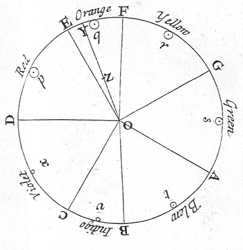
Newton’s_color_circle (Newton, 1704).

Establishing invariance in the psychological space

What is sometimes required is not more data or more refined data but a different conception of the problem.

Assume the invariant law of generalization is based on an appropriate psychological space Attribute the troublesome variations in the generalization gradients to variations in a psychophysical function (physical space $\rightarrow$ psychological space) A purely psychological function relates generalization to distance in the psychological space.

Is there an invariant monotonic function whose inverse will uniquely transform those data into numbers interpretable as distances in some appropriate metric space?

Goal: find a metric space (or, the inverse function) that explains the observed generalization data(Satisfying certain conditions like certain Cayley-Menger determinants https://en.wikipedia.org/wiki/Cayley%E2%80%93Menger_determinant)

• Uniqueness implied by geometric fact: rank order of distance can be a good approximation to the distances, when the number of points is not too small (relative to dimensionality)
• The function can be determined through nonmetric multidimensional scaling
  • move $n$ points in a specified space, until the configuration minimizes some measure of departure (“stress”) from a monotonic relation between $g_{ij}$ and $d_{ij}$. \(g_{ij}=\bigg(\frac{p_{ij}\cdot p_{ji}}{p_{ii}\cdot p_{jj}}\bigg)^{1/2}\)

Empirical regularities

Invariance and (approximate) exponential decay

Invariance: in every case, the decrease of generalization with psychological distance is

1. monotonic,
2. generally concave upward, and
3. more or less approximates a simple exponential decay function

MDS does not impose the form of function except for monotonicity.

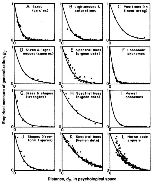
Gradients of generalization (Shepard, 1987).

Two distance metrics

When the psychological space has more than 1 dimension, data also provide evidence about the metric for unitary and analyzable stimuli

• integral attributes (lightness and saturation) : Euclidean metric
• separable attributes (size and orientation): ‘city-block’ metric They can be expressed as a Minkowski power metric \(d_{ij}=\bigg(\sum_{k=1}^K|x_{ik}-x_{jk}|^r\bigg)^{1/r}\)

A theory of generalization

Generalization is thus a cognitive act, not merely a failure of sensory discrimination.

Recognition as member of a “Natural kind”, corresponding to some consequential region $C$ in the psychological space.

Assumption: nature chose the consequential region at random

1. all locations are equally probable
2. size has density $p(s)$ with finite mean $\mu$ \(\int_0^\infty p(s)ds =1\,E[s]=\int_0^\infty s\cdot p(s)ds = \mu<\infty\)
3. arbitrary shape that is centrally symmetric and has finite extension

Goal: estimate the conditional probability $P\big(x\in C\vert 0\in C)$

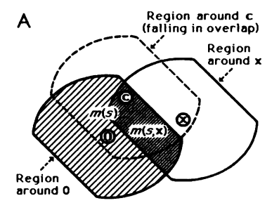
Consequential regions with fixed size (Shepard, 1987).

Given any size $s$, the probability of covering $x$ is the ratio of the volunetric measure. \(p(x\in C\vert s)=\frac{m(s,x)}{m(s)}\)

Marginalize out size to derive the conditional probability, denoted as $g(\cdot)$. Note that $p(\cdot)$ satisfies some conditions. \(g(x)=\int_0^\infty p(s)\frac{m(s,x)}{m(s)}ds\)

Exponential Law

Derivation with unidimensional case

A convex consequential region is an interval of a certain length \(m(s)=s\) \(m(s,x)=\left\{\begin{array}{ll} s-\vert x\vert,& s\geq \vert x\vert \\ 0, & s<\vert x\vert \end{array}\right.\)

Taking these into the previous expression, and taking derivatives lead to \(g''(d)=\frac{p(d)}{d}\)

Some simulation results with different size distribution

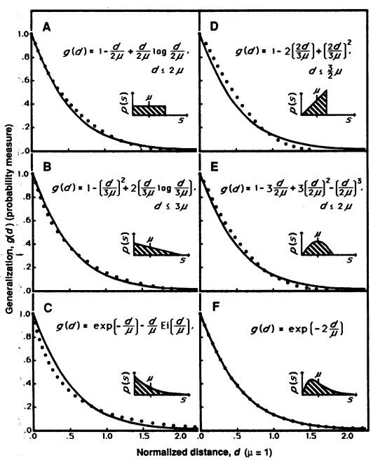
Generalization function and corresponding prior (Shepard, 1987).

• dependence on the prior is weak
• exponential law is exact under Erlang prior $p(s)=(\frac{2}{\mu})^{2}s\cdot \exp(\frac{-2}{\mu}s)$ \(g(d) = \exp\bigg(-2\frac{d}{\mu}\bigg)\)
• Erlang prior can be derived using Baysian update of prior assuming minimum knowledge (the first stimulus falls in the consequential region with probability proportional to its volumn $m(s)$) \(p(s)=C\cdot m(s) \cdot q(s)\)

  Derivation of two metrics

  For multidimensional cases, different metrics can be considered as a result of different dependence relations between dimensions.

• For dimensions identified as independent variables in the world, extension of consequential region along these dimensions should not be correlated

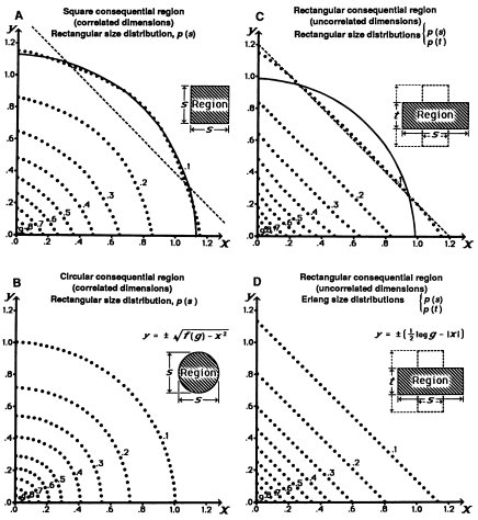
Equal generalization contours (Shepard, 1987).

Limitations

• When tested on highly similar stimuli, or in delayed test, “noise” will come into effect
  1. exponential decay $\rightarrow$ Gaussian (Shepard, 1987: fig.1 L)
  2. rhombic $\rightarrow$ elliptical curve of equal generalization for analyzable dimensions
• Effect of category learning; asymmetries of generalization
• Alternative explanations based on graded generalization form of consequential region
• Negative correlation of dimensions lead to $r<1$
• Time to discriminate reciprocally related to distance, not exponentially

Howard, R. A., & Matheson, J. E. (1972). Risk-sensitive Markov decision processes. Management science, 18(7), 356-369.

This paper provides formulation and algorithm for the maximization of certain equivalent reward (utility) generated by a MDP.

• The eigenvalue of $Q$, $\lambda$, may (?) be used to elicitated risk attitude $\gamma$

Definitions and notations

$\tilde{v}$ is the certain equivalent of a lottery with outcome $v$, $u(v)=u(\tilde{v})$

Denote $u_i(n)=u(\tilde{v}_{i}(n))$ be the utility of the reward process when it occupies state $i$ and there are $n$ periods left.

Assumption

Assume delta property, that when all prizes in a lottery increases by the same amount, certain equivalent increases by the same amount.

• To ensure this property, the utility function has to be either linear or exponential

The exponential utility implies a constant increase in lottery will become a multiplicative term \(u(v+\Delta)=e^{-\gamma \Delta} u(v)\)

Formulation

Reward process

Stationary MRP

Equivalently, we can use matrix notation, $Q_{ij}=p_{ij}e^{-\gamma r_{ij}}$

\(\text{u}(n)=Q^{n}\text{u}(0)\) We can show that, \(\lim_{n\rightarrow \infty}[\tilde{v}_{i}(n)-n(- \frac{1}{\gamma} \ln\lambda)]=\tilde{v}_{i}+c\)

• $\lambda$ is the first eigen value of $Q$
• $\tilde{v}_{i}$ is the relative certain equivalent
• $\tilde{g}=- \frac{1}{\gamma} \ln\lambda$ is the certain equivalent gain

We can re-write the consistency condition

Decision process

\(u_{i}(n+1)=\max_{k}\sum\limits_{j} p_{ij}^{k}(n+1)e^{-\gamma r^{k}_{ij}(n)} u_j(n)\)

• this equation allows us to compute the optimal policy and the optimal utility
• We can also find $\tilde{v}_{i}(n)$, the certain equivalent of the lottery implied by being in state $i$ with $n$ stages left

Algorithm for stationary policy

policy evaluation: for the present policy, solve

with $\tilde{v}_{N}=0$, for certain equivalent gain $\tilde{g}$ and the relative certain equivalents.

policy improvement: For each state $i$ find the alternative $k$ that maximizes the certain equivalent

Jaquette, S. C. (1976). A utility criterion for Markov decision processes. Management Science, 23(1), 43-49.

Utility criterion

The following utility criterion is used \(u(X)=-\exp(-\sum\limits_{t}\lambda_{t}x_{t}),\) where $\lambda_{t}= \lambda \beta^{t}$, reflecting time discount and constant risk averse.

• The function form is log-additive (pollack, 1967)
• It also satisfies risk independence
• The formulation can be considered also as a utility function of the total reward, discounted to the current period

Utility optimality

A policy $\pi=(f_1,…,f_t,…)$ is a sequence of vectors. $f_t=\pi_t(s_t)$ maps from states to actions.

• A policy $\pi^{*}$ is utility optimal with constant risk aversion $\lambda$ if $u_{\pi^{*}}(\lambda)\geq u_{\pi}(\lambda)$ for all $\pi$.
• A policy $\pi=(f_1,…,f_t,…)$ is ultimately stationary if $f_t=f$ for all $t$ larger than some finite integer

Thm. A utility optimal policy $\pi^{*}(\lambda,\beta)$ exists for all $\lambda\geq 0$ and all $0\leq\beta<1$ which is ultimately stationary. The policy $\pi^{*}$ can be chosen as a piecewise constant function of $\lambda$ and $\beta$, with an ultimate action vector $f$ a piecewise constant function of $\beta$ only (and constant for all $\beta$ close to 1).

• stationary policies are not utility optimal generally.

Rusmevichientong, P., & Tsitsiklis, J. N. (2010). Linearly parameterized bandits. Mathematics of Operations Research, 35(2), 395-411.

The key ideas for finding bounds is to

• attribute regret to the causes: exploration or estimation error
• find the relation between these two parts, if any

Model formulation

$\mathcal{U}_r \subset \mathbb{R}^r$ a compact set if arms ($r\geq2$), The reward in period $t$ is given by

\(X_{t}^{u}=u^{T}Z + W_{t}^{u},\tag{1}\)

• $Z\in\mathbb{R}^r$ is a random variable
• $W_{t}^{u}$ are iid mean-zero random variables

A policy $\psi=(\psi_{1},\psi_{2},…)$ is a sequence of functions, each mapping from history to $\mathcal{U}_r$. For any policy $\psi$ and $z\in\mathbb{R}^r$, the cumulative regret under $\psi$ given $Z=z$ is

The cumulative Bayes risk under $\psi$ is the expectation w.r.t. the prior of $Z$.

Lower bounds

Linear bandits has $\Omega(r\sqrt{T})$ lower bounds on the Bayes risk and thus on regret, given normal prior on $Z$.

1. The cumulative risk can be lower-bounded by the estimator error variance and the total amount of exploration.

   Lemma (risk decomposition) Let $S_{t}^{1},…, S_{t}^{r-1}$ denote a collection of orthogonal unit vectors that are also orthogonal to $\hat{Z}$. For any $T\geq 1$, \(\text{Risk}(T,\psi)\geq \frac{1}{2}\sum\limits_{k=1}^{T}E \bigg[||Z||\sum\limits_{t=1}^{T}(T_{t}^{T}S_{t}^{k})^{2} + \frac{T}{||Z||} \{(Z-\hat{Z}_{T})^{T}S_{T}^{k}\}^2\bigg]\)

2. The two terms are interelated. Little exploration implies large estimation error

   Lemma For any $k$ and $T\geq 1$, \(E[\{(Z-\hat{Z})^{T}S_{T}^{k}\}^{2}\vert H_{T}]\geq\frac{1}{r+\sum\limits_{t=1}^{T}(T_{t}^{T}S_{t}^{k})^{2} },\) where $r$ is prior precision of $Z$.

3. There is a lower bound on the probability that $Z$ is bounded away from 0.
4. Then we can derive a minimum directional risk.

Upper bounds: PEGE algorithm

Algorithm: phased-exploration-and-exploitation

There are two phases in each cycle $c\geq 1$:

1. Exploration ($r$ periods) play arm $b_k$. The explored arms span the entire space. compute the OLS estimate $\hat{Z}(c)=Z+\frac{1}{c}(\sum\limits_{k=1}^{r}b_{k}b_{k} ^{T})^{-1}\sum\limits_{s=1}^{c}\sum\limits_{k=1}^{r}b_{k}W^{b_{k}}(s)$
2. Exploitation ($c$ periods) play the greedy arm $G(c)=\arg\max_{v\in\mathcal{U}_{r}} v^{T}\hat{Z}(c)$. In the algorithm, $c$ is of the order $O(\sqrt{T})$.

Assumptions

1. Subgaussian noise
2. Arms are bounded, and include $r$ linearlly independent components
3. $\mathcal{U}_{r}$ satisfy smooth best arm response with parameter J \(||u^{*}(z)-u^{*}(y)||\leq J||z-y||\)

Upper bound

For PEGE, we can explicitly disentangle risk caused by exploration and misspecification

Thm. There exists a positive constant $a_{1}$ that depends only on the noise bounds, arm bounds and response bounds, such that for any $z$ and $T\geq r$, \(\text{Regret}(z,T,\text{PEGE})\leq a_{1}(||z||+\frac{1}{||z||})r\sqrt{T}\)

• Since the arm bound provides a trivial bound $2\bar{u}\vert\vert z\vert\vert$ on instantaneous regret, the bound does not deteriorate as $\vert\vert z\vert\vert$ approaches 0.

Proof sketch:

1. There is an upper bound on the squared norm error \(E[||\hat{Z}(c)-z||^{2}| Z=z]\leq \frac{h_{1}r}{c}\)
2. Expected instantaneous regret under greedy decision is of order $O(\vert\vert Z-\hat{Z}\vert\vert^{2})$ given smoothness assumption.
3. Over total $K$ cycles, $K=O(\sqrt{T})$ \(\text{Regret}\left(z,rK+\sum\limits_{c=1}^{K}c,\text{PEGE}\right)\leq h_{3}r||z||K+h_{4}\sum\limits_{c=1}^{K} \frac{r}{||z||}\)

Pollak, Robert A. “Additive von Neumann-Morgenstern utility functions.” Econometrica 35.3/4 (1967): 485-494.

Axiomatically characterize the class of (log-)additive utility functions with axioms on preferences.

Definitions and notations

Utility function forms

A vNM utility functionis ordinally additive if there exist $T$ functions $v^t(x_t)$ and a twice differentiable function $F$, $F’>0$, such that $F[V(X)]=\sum\limits_{t=1}^{T} v^t(x_t)$.

• A log-additive utility function is ordinally additive.

Alternatives: lottery tickets

Let $X_a,Y_a$ be $T$-dimensional vector representing consumption paths:$X_a=(x_{a1},…,x_{aT}), Y_a=(y_{a1},…,y_{aT})$, and let $\gamma_a\in[0,1]$ be a number. A simple lottery ticket $L_a=(\gamma_a,X_a,Y_a)$ is an alternative that, once chosen, yields $X_a$ with probability $\gamma_a$ and $Y_a$ with probability $1-\gamma_a$. \(V(L_{a}) = \gamma_{a} V(X_{a}) + (1-\gamma_{a}) V(Y_a)\)

• Two simple lottery tickets $L_a,L_b$ are a pair of k-standard lottery tickets $(L_a,L_b)$ if (1) $\gamma_a=\gamma_b=\frac{1}{2}$, and (2) have a common value on the first consumption path $x_{ak}=x_{bk}=x_k$.
• Two simple lottery tickets $L_a,L_b$ are a pair of k-normal lottery tickets $\langle L_a,L_b\rangle$ if (1) $\gamma_a=\gamma_b=\frac{1}{2}$, and (2) have a common value on both consumption paths $x_{ak}=x_{bk}=y_{ak}=y_{bk}=z_k$.

Characterization theorems

Strong additivity axiom: an individual’s preference between two k-standard lottery tickets in a given pair is independent of the level of $x_k$ for all pairs of k-standard lotteries, and all choice of $k$.

• If $V(L_a(x_k))>V(L_b(x_k))$ for some $x_k$, then $V(L_a(x_k’))>V(L_b(x_k’))$ for all $x_k’$.

Thm 1. An individual’s preferences satisfy the strong additive axiom if and only if his von Neumann-Morgenstern utility function is additive.

• proof sketch: construct two consumption paths, and differentiate the utility functions with repect to $k$.This gives an equation showing that $\partial V(X) / \partial x_k$ depends only on $x_k$. The necessity part is trivial.

Weak additivity axiom: an individual’s preference between two k-normal lottery tickets in a given pair is independent of the level of $z_k$ for all pairs of k-normal lotteries, and all choice of $k$.

• If $V(L_a(z_k))>V(L_b(z_k))$ for some $z_k$, then $V(L_a(z_k’))>V(L_b(z_k’))$ for all $z_k’$.
• Weak additivity axiom is weaker in the sense that, it restricts preference on k-normal lotteries, which is a subset of k-standard lotteries.

Thm 2. An individual’s preferences satisfy the weak additive axiom if and only if his von Neumann-Morgenstern utility function is additive or log-additive.

• proof sketch: to show the suficient condition, a lemma points out (by construction) that weak additivity implies ordinally additive property. By differentiating two indifferent consumption paths with respect to $x_k$, we can show that $H’(V)=G’‘(S)/G’(S)=c$ is a constant. This shows that $G$ must be a linear or exponential transformation.

Implications for sequential decision making

Consider the preference satisfying weak additivity axiom: \(V(x_1,...,x_T)=G(\sum\limits_{t=1}^{T}v^t(x_t)),\) where $G$ is a linear or exponential transformation.

• A single choice is made between different streams of income
• Q: why should the decision maker considers reward in each period independently.

Pratt, John W. “Risk Aversion in the Small and in the Large.” Econometrica 32.1/2 (1964): 122-136.

For the utility functions for money, a local risk measure is defined. (equation (3))

• The risk premium can be locally represented using the local risk aversion. (equation (2))
• This measure is closely related to global risk-averse preferences.

Definitions and notations

• $u_{1}(x)\sim u_{2}(x)$: two functions are equivalent as utilities (up to increasing linear transformation)
• $\pi({x,\tilde{z}})$: the risk premium (elaborated below)

The risk premium $\pi$

Given assets $x$ and utility function $u$, a decision maker is indifferent between receiving a risk $\tilde{z}$ and the non-random amount $E[\tilde{z}]-\pi$. Mathematically, \(u(x+E(\tilde{z})-\pi(x,\tilde{z}))=E[u(x+\tilde{z})].\tag{1}\)

• From equation (1) the risk premium is uniquely defined.
• It follows from (1) that for any constant $\mu$, $\pi(x,\tilde{z})=\pi(x+\mu,\tilde{z}-\mu)$. Therefore, we may only consider any actuarially neutral risk.

There are other related concepts like the cash equivalent and insurance premium. These concepts should be distinguished from the bid price.

Local risk aversion

Consider $\pi(x,\tilde{z})$ for an actuarially neutral risk $\tilde{z}$ with infinitesimal variance $\sigma_z^2{\rightarrow}0$. Locally expand equation (1) on both sides shows \(\begin{equation} \begin{split} u(x-\pi)&=u(x)-\pi u'(x) + O(\pi^2)\\ E[u(x+\tilde{z})]&=E[u(x)+\tilde{z}u'(x)+\frac{1}{2}\tilde{z}^2u''(x)+O(\tilde{z}^3)]\\ &=u(x)+\frac{1}{2}\sigma_z^2u''(x)+o(\sigma_z^2) \end{split} \end{equation}\)

Setting equal these equations gives \(\pi(x,\tilde{z})=\frac{1}{2}\sigma_z^{2}r(x)+ o(\sigma_z^2),\tag{2}\) where \(r(x)=-\frac{u''(x)}{u(x)}=-\frac{d}{dx}\log u'(x). \tag{3}\)

• There is a similar interpretation with discrete risks and probability premium $p(x,h)=p(\tilde{z}=h)-p(\tilde{z}=-h)$.

Relation with utility function

The local risk aversion function $r$ associated with any utility function $u$ contains all essntial information about $u$.

Equation (3) implies \(u\sim\int e^{-\int r} \tag{4}\)

• It can be convenient to preserve $u$ since it determines ordinary (as against infinitesimal) risk preferences.

Concavity

$u$’’$(x)$ is not in itself a meaningful measure of concavity in utility theory

• the sign of $u$’’$(x)$ implies general attitude towards risk
• the absolute magnitude is not meaningful

Comparative (global) risk aversion

If $r_1(x)>r_2(x)$, then $u_1$ is more risk-averse than $u_2$ at $x$ not only locally, but also globally. Thm. Let $r_i(x),\pi_i(x)$ be the local risk aversion and risk premium according to the utility function $u_i,\,i=1,2$. Then the following conditions are equivalent:

1. $r_{1}(x)\geq r_2(x)$ for all $x$
2. $\pi_1(x,\tilde{z})\geq \pi_2(x,\tilde{z})$ for all $x$ and $\tilde{z}$
3. $u_1(u_2^{-1}(t))$ is a concave function of $t$
4. $\frac{u_1(y)-u_1(x)}{u_1(w)-u_{1(v)}} \leq \frac{u_2(y)-u_2(x)}{u_2(w)-u_2(v)}$ for all $v<w\leq x<y$.

• condition 1. requires local risk-aversion to be larger for any asset.

Special family of risk aversion

Constant risk aversion

If the local risk aversion is constant $r(x)=c$, then

• If the risk aversion is constant locally, then it is also constant globally. For any $k,\,u(x+k)\sim u(x)$.

Decreasing risk aversion

Decreasing risk aversion describes a decision maker, who (1) attaches positive risk premium (risk-averse) to any risk, but (2) attaches smaller risk premium the greater his assets $x$. Formally,

1. $\pi(x,\tilde{z})>0$ for all $x$ and $\tilde{z}$
2. $\pi(x,\tilde{z})$ is a strictly decreasing function of $x$ for all (given) $\tilde{z}$

Decreasing global risk aversion is equivalent to decreasing local risk aversion,i.e. the following conditions are equivalent

1. The local risk aversion $r(x)$ is decreasing
2. The risk premium $\pi(x,\tilde{z})$ is a decreasing function of $x$ for all $\tilde{z}$